Recipes

Whole paranome inference

Here we used the real coding sequence data of a basal eudicot, Aquilegia coerulea to conduct the analysis. The command we used is as below.

(ENV)$ wgd dmd Aquilegia_coerulea

By default, the output directory is named as wgd_dmd locating at the same directory as the script. The output file name inside is Aquilegia_coerulea.tsv. In short, the workflow of this step is diamond + normalization + mcl, as shown below.

K_S distribution construction

To build the K_S distribution, with the paralogous gene families inferred above, we use the command below.

(ENV)$ wgd ksd wgd_dmd/Aquilegia_coerulea.tsv Aquilegia_coerulea

The anchor K_S distribution can be further constructed by the program wgd syn with the command below.

(ENV)$ wgd syn -f mRNA -a Name wgd_dmd/Aquilegia_coerulea.tsv Aquilegia_coerulea.gff3 -ks wgd_ksd/Aquilegia_coerulea.tsv.ks.tsv

Synteny inference

Associated with the anchor K_S distribution, there are some other probably interesting syntenic plots also being produced from the command above. One is the Syndepth plot shown below, which reflects that A. coerulea has numerous duplicated collinear segments and a few triplicated collinear segmentsretained.

Besides, the dupStack plot shows more intuitively the distribution of duplicated segments across the chromosomes.

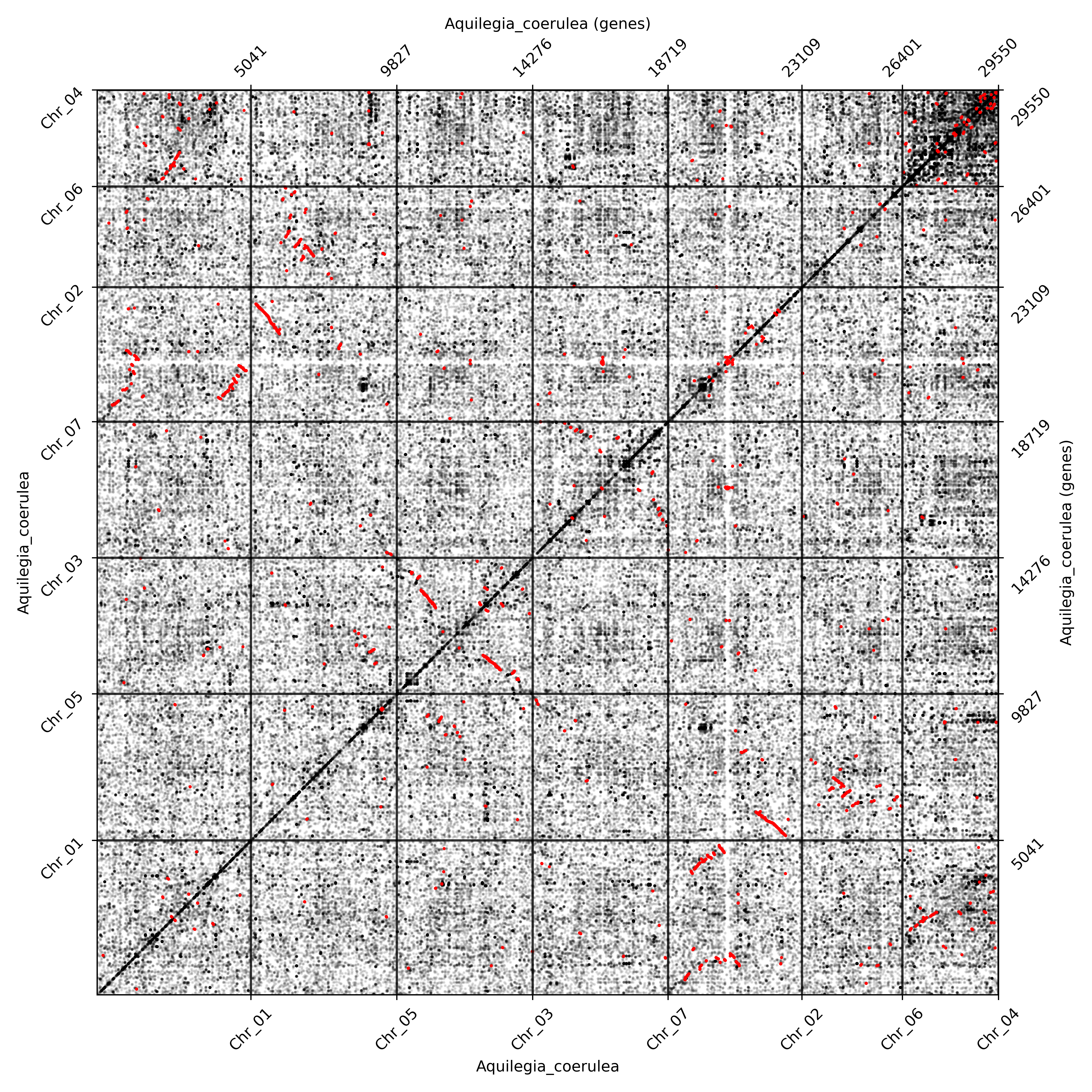
The dotplot in oxford grid in the unit of nucleotides and genes will also be automately produced with K_S annotated.

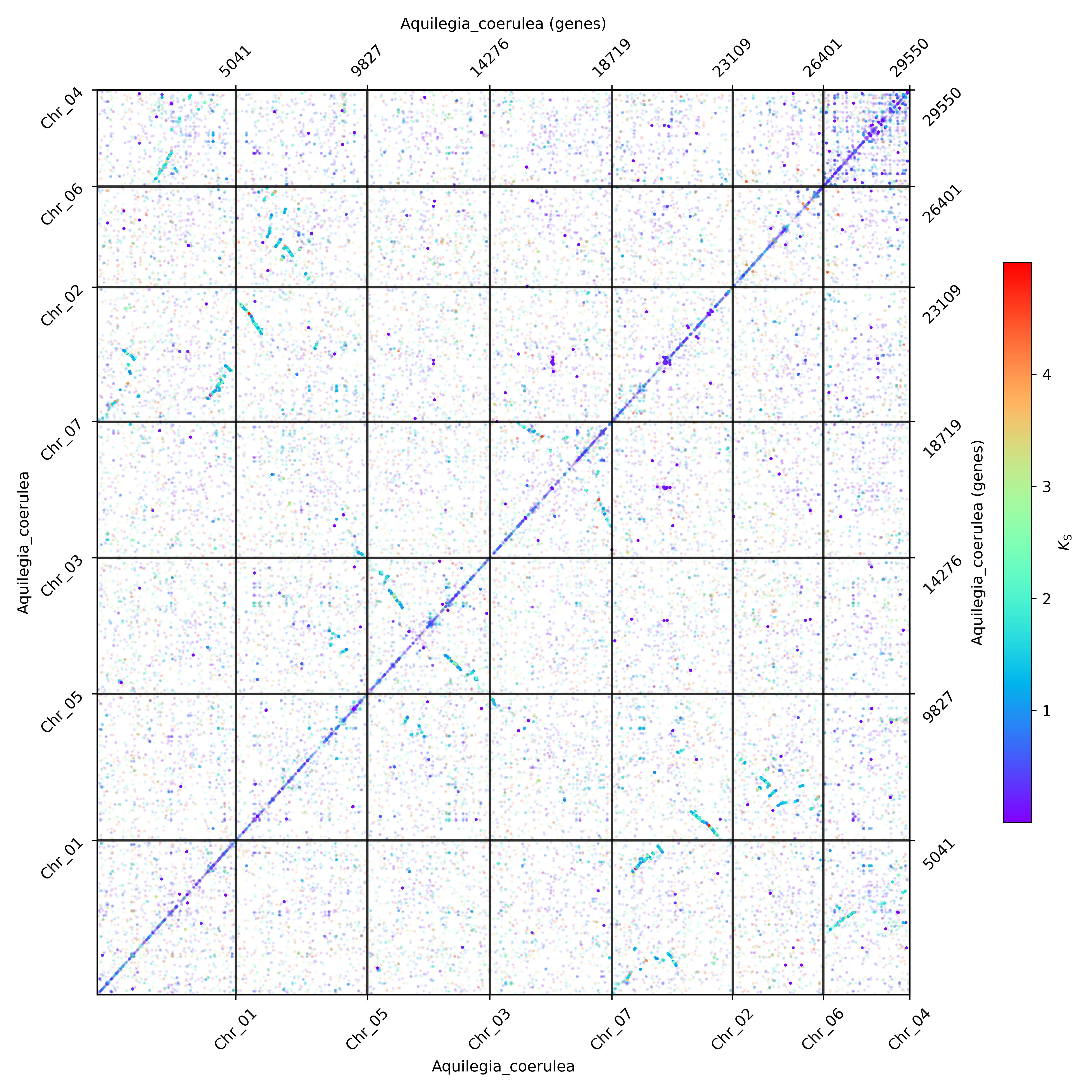
The ones above are with K_S annotation, the ones without K_S annotation are as below.

Note

The opacity of anchor dots and all homolog dots can be set by the option apalpha and hoalpha separately. If one just wants to see the anchor dots, setting the hoalpha as 0 (or other minuscule values) will do. If one wants to see the distribution of whole dots better, setting the hoalpha higher (and apalpha lower) will do. The dotsize option can be called to adjust the size of dots.

Mixture modeling

To gain a model-based view of when there might be likely WGD peaks, we can conduct an exponential-lognormal mixture modeling (ELMM) using the command below.

(ENV)$ wgd viz -d wgd_ksd/Aquilegia_coerulea.tsv.ks.tsv

Above we just did a mixture modeling analysis for the whole paranome, we can do another Gaussian mixture modeling upon the anchor K_S using the command below.

(ENV)$ wgd peak wgd_ksd/Aquilegia_coerulea.tsv.ks.tsv --anchorpoints wgd_syn/iadhore-out/anchorpoints.txt --segments wgd_syn/iadhore-out/segments.txt --listelements wgd_syn/iadhore-out/list_elements.txt --multipliconpairs wgd_syn/iadhore-out/multiplicon_pairs.txt --weighted

Substitution rate correction

On the whole, the likely WGD peak around the K_S age 1.2 and numerous duplicated collinear segments suggest a paleo-polyploidization event. To resolve its phylogenetic location, for instance, whether it’s shared by all eudicots or limited to A. coerulea, we can conduct a rate-correction analysis and directly compare the relative timing of polyploidization and speciation event. To achieve the goal, we firstly have to calculate the orthologous K_S distribution, using the command below.

(ENV)$ wgd dmd --globalmrbh Aquilegia_coerulea Protea_cynaroides Acorus_americanus Vitis_vinifera -o wgd_globalmrbh
(ENV)$ wgd ksd wgd_globalmrbh/global_MRBH.tsv --extraparanomeks wgd_ksd/Aquilegia_coerulea.tsv.ks.tsv -sp speciestree.nw --reweight -o wgd_globalmrbh_ks --spair "Aquilegia_coerulea;Protea_cynaroides" --spair "Aquilegia_coerulea;Vitis_vinifera" --spair "Aquilegia_coerulea;Acorus_americanus" --spair "Aquilegia_coerulea;Aquilegia_coerulea" --plotkde (-ap wgd_syn/iadhore-out/anchorpoints.txt)

The first wgd dmd command is to infer the global MRBH families as preparatory files. The second wgd ksd command is doing two things, 1) calculating the orthologous K_S values and 2) conducting rate-correction. Here the users are required to provide explicitly the species pairs to be plotted and the species tree file in newick format to properly conduct rate-correction. The anchor pairs information can be optionally provided by using the option anchorpoints.

Substitution rate correction with mixture modeling

If one wants to combine the ELMM modeling result with the rate-correction result, it is very easy to achieve. Just add one more option plotelmm.

(ENV)$ wgd viz -d wgd_globalmrbh_ks/global_MRBH.tsv.ks.tsv --extraparanomeks wgd_ksd/Aquilegia_coerulea.tsv.ks.tsv -sp speciestree.nw --reweight -ap wgd_syn/iadhore-out/anchorpoints.txt -o wgd_viz_mixed_Ks_elmm --spair "Aquilegia_coerulea;Protea_cynaroides" --spair "Aquilegia_coerulea;Vitis_vinifera" --spair "Aquilegia_coerulea;Acorus_americanus" --spair "Aquilegia_coerulea;Aquilegia_coerulea" --gsmap gene_species.map --plotkde --plotelmm

Note

The substitution rate correction process can be achieved by either wgd ksd or wgd viz. The difference is that wgd ksd will conduct the basic K_S estimation anyway. So the recommended way will be first calculating all the required K_S values, including paralogues and orthologues K_S, and then calling wgd viz to do the rate correction and plot. The additional required file gene_species.map is automately produced from the wgd ksd step. But it’s also easy to manually prepare the map file. The format is as below. The separator is space instead of tab.

Aqcoe6G057800.1 Aquilegia_coerulea
Vvi_VIT_201s0011g01530.1 Vitis_vinifera
Pcy_Procy01g08510 Protea_cynaroides
Aam_Acora.04G142900.1 Acorus_americanus

Another possible layer is the mixture modeling result of anchor K_S, which can be added simply by the option plotapgmm.

(ENV)$ wgd viz -d wgd_globalmrbh_ks/global_MRBH.tsv.ks.tsv --extraparanomeks wgd_ksd/Aquilegia_coerulea.tsv.ks.tsv -sp speciestree.nw --reweight -ap wgd_syn/iadhore-out/anchorpoints.txt -o wgd_viz_mixed_Ks_elmm --spair "Aquilegia_coerulea;Protea_cynaroides" --spair "Aquilegia_coerulea;Vitis_vinifera" --spair "Aquilegia_coerulea;Acorus_americanus" --spair "Aquilegia_coerulea;Aquilegia_coerulea" --gsmap gene_species.map --plotkde --plotelmm --plotapgmmm

So far, we can see that the WGD peak of A. coerulea is 1.19 for whole paranome and 1.28 for anchor pairs, younger than the corrected divergence peak with Protea cynaroides and Vitis vinifera, suggesting that the WGD event should happen after the divergence event, thus a lineage-specific WGD of A. coerulea. The saying “lineage-specific” is a relative concept that it might be shared by other species too, just not the species involved here. In fact, this WGD event is showed to be shared by all Ranunculales by other studies which sampled more Ranunculales species for comparison.

Multiple orthologous K_S distribution

If one just wants to plot the orthologus K_S distributions for multiple species pair, it’s also easy to achieve. Just don’t add the paralogous species pair Aquilegia_coerulea;Aquilegia_coerulea. An example command is as below.

(ENV)$ wgd viz -d wgd_globalmrbh_ks/global_MRBH.tsv.ks.tsv -sp speciestree.nw --reweight -o wgd_viz_Compare_rate --spair "Acorus_americanus;Protea_cynaroides" --spair "Aquilegia_coerulea;Acorus_americanus" --spair "Vitis_vinifera;Acorus_americanus" --gsmap gene_species.map --plotkde

To sum up a little bit, the logic of this mixed K_S distribution part is to diy the plot by adding different layers, including plotelmm, plotapgmm, and --plotkde which controls whether to add the kde curve of orthologus K_S distributions.

WGD dating

Above we discussed about the identification and phylogenetic placement of WGDs. An absolute dating of WGD can also be achieved in three more steps. The first step is to select the anchor pairs used in orthogroup construction. An example command is as below.

(ENV)$ wgd peak --heuristic wgd_ksd/Aquilegia_coerulea.tsv.ks.tsv -ap wgd_syn/iadhore-out/anchorpoints.txt -sm wgd_syn/iadhore-out/segments.txt -le wgd_syn/iadhore-out/list_elements.txt -mp wgd_syn/iadhore-out/multiplicon_pairs.txt -o wgd_peak

This step we firstly detect possible peaks emerged in the anchor K_S distribution. Then, the properties associated with the peak, i.e., the location and the half width will be used as the mean and standard deviation of the assumed log-normal distribution. The 95% confidence level of this log-normal distribution will be used to constrain the anchor pairs for dating. For instance, the output file Aquilegia_coerulea.tsv.ks.tsv_95%CI_AP_for_dating_weighted_format.tsv is the selected anchor pairs for dating. The second step is to construct the orthogroups used in molecular dating. The command is as below.

(ENV)$ wgd dmd -f Aquilegia_coerulea -ap wgd_peak/Aquilegia_coerulea.tsv.ks.tsv_95%CI_AP_for_dating_weighted_format.tsv -o wgd_dmd_ortho Potamogeton_acutifolius Spirodela_intermedia Amorphophallus_konjac Acanthochlamys_bracteata Dioscorea_alata Dioscorea_rotundata Acorus_americanus Acorus_tatarinowii Tetracentron_sinense Trochodendron_aralioides Buxus_austroyunnanensis Buxus_sinica Nelumbo_nucifera Telopea_speciosissima Protea_cynaroides Aquilegia_coerulea

This step requires users to design a starting tree used in mcmctree dating. The one we use is as below. The orthogroups constructed are actually the local MRBHs intersected with the given anchor pairs, where the focus species is A. coerulea.

17 1
((((Potamogeton_acutifolius,(Spirodela_intermedia,Amorphophallus_konjac)),(Acanthochlamys_bracteata,(Dioscorea_alata,Dioscorea_rotundata))'>0.5600<1.2863')'>0.8360<1.2863',(Acorus_americanus,Acorus_tatarinowii))'>0.8360<1.2863',((((Tetracentron_sinense,Trochodendron_aralioides),(Buxus_austroyunnanensis,Buxus_sinica))'>1.1080<1.2863',(Nelumbo_nucifera,(Telopea_speciosissima,Protea_cynaroides)))'>1.1080<1.2863',(Aquilegia_coerulea_ap1,Aquilegia_coerulea_ap2))'>1.1080<1.2863')'>1.2720<2.4720';

It’s mandatory to set the focus species, i.e. A. coerulea, to be as “Aquilegia_coerulea_ap1” and “Aquilegia_coerulea_ap2”, such that the program knows which node to retreive information. In fact, the column names in the file merge_focus_ap.tsv also include “Aquilegia_coerulea_ap1” and “Aquilegia_coerulea_ap2”. The final step, also the real dating step, can be achieved by the command below.

(ENV)$ wgd focus --protdating --aamodel lg wgd_dmd_ortho/merge_focus_ap.tsv -sp dating_tree.nw -o wgd_dating -d mcmctree -ds 'burnin = 2000' -ds 'sampfreq = 1000' -ds 'nsample = 20000' Potamogeton_acutifolius Spirodela_intermedia Amorphophallus_konjac Acanthochlamys_bracteata Dioscorea_alata Dioscorea_rotundata Acorus_americanus Acorus_tatarinowii Tetracentron_sinense Trochodendron_aralioides Buxus_austroyunnanensis Buxus_sinica Nelumbo_nucifera Telopea_speciosissima Protea_cynaroides Aquilegia_coerulea

To only conduct the peptide concatenation-based dating, we add the flag protdating. The model we use is the lg model. We set the sample number as 20000 and the sample frequency as 1000, with first 2000 samples as burn-in, thus in total 20002000 iterations to ensure convergence. To visualize the date, we provide a python script postplot.py stored in the wgd folder to plot the WGD dates. Its usage is as below.

(ENV)$ python postplot.py postdis dates.txt --percentile 90 --title "WGD date" --hpd -o "Ranunculales_WGD_date.svg"

Note

Users need to manually prepare the dates.txt file for plotting. It’s the 20000 samples from the output file mcmc.txt. The format is as below.

t_n33
1.1837082
1.1248203
1.2071548
...

The final WGD date is as shown below, whose posterior mean, median and mode are 112.92, 113.44 and 112.54 mya respectively, with 90% HPD as 105.07 - 122.32 mya.

The whole workflow of dating can be simplified as below.